Unlike the common belief, being a theoretical physicist nowadays is not just solving equations. In fact, my research requires me to do a lot of programming. Here is a selected list of codes that I have developed as part of my research.
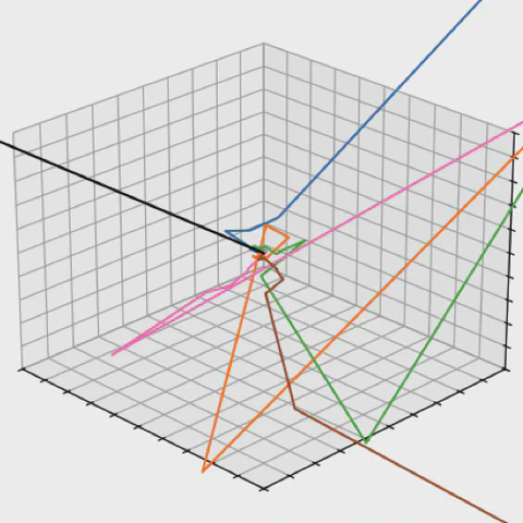
SPaRTA 🛡️ = SPeedy Lyman alpha Ray Tracing Algorithm. The code can be used to perform quickly MC simulations of the trajectories of absorbed Lyman alpha photons in the intergalactic medium (IGM), plotting them, and gather insights on their properties. Let us look for example on the trajectories of 6 photons as they travel through the IGM, until they are absorbed at the center at redshift $z_\mathrm{abs}=10$. The black line in all plots corresponds to a photon traveling in a straight-line. On large scales, all photons appear to travel in straight-lines as their aparent frequency is far away from the Lyman alpha line center. On small scales, the photons appear to do a random walk with a step size that decreases as we zoom-in, this happens as on the smallest scales the frequency of the photons is close to Lyman alpha and the cross-section for interacting with the hydrogen atoms in the IGM becomes very large. The diffustion scale is the intermediate scale that separates “large” scales and “small” scales. It can be analytically estimated to be $$r_{*}\left(z_\mathrm{abs}\right)\approx10\,x_{\mathrm{HI}}\left(\frac{\Omega_{b}h^{2}}{0.0223}\right)\left(\frac{\Omega_{m}h^{2}}{0.143}\right)^{-1}\left(\frac{1-Y_{\mathrm{He}}}{0.755}\right)\left(\frac{1+z_{\mathrm{abs}}}{10}\right)\,\mathrm{Mpc}.$$We can see indeed that the photons change their behavior when we plot their distance and frequency from the origin as a function of time (or redshift). The dotted lines below mark the diffusion scale. Interstingly, when studying the radial distribution of the photons from the origin, given absorption redshift $z_\mathrm{abs}$ and emission redshift $z_\mathrm{em}$, the distribution depends mainly on $x_\mathrm{em}\equiv R_\mathrm{SL}\left(z_\mathrm{abs},z_\mathrm{em}\right)/r_{*}\left(z_\mathrm{abs}\right)$, where $R_\mathrm{SL}\left(z_\mathrm{abs},z_\mathrm{em}\right)$ is the comoving distance between $z_\mathrm{abs}$ and $z_\mathrm{em}$. This quantity can be thought of as the comoving distance between absorber and emitter, normalized by the diffusion scale. So for $x_\mathrm{em}\gg 1$, the distribution tends towards $\delta\left(r-R_\mathrm{SL}\right)$, reflecting the straight-line limit, while for $x_\mathrm{em}\ll 1$, the distribution shifts more towards smaller distances. These distributions can be fitted nicely to beta distributions, $f\left(r\right)\propto r^{\alpha-1}\left(R_\mathrm{SL}-r\right)^{\beta-1}$. When $x_\mathrm{em}\gg 1$ we have $\alpha\gg\beta$, while $x_\mathrm{em}\ll 1$ corresponds to $\alpha\ll\beta$.
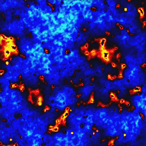
21cmFirstCLASS is an extension of the popular 21cmFAST code that interfaces with CLASS to generate initial conditions at recombination that are consistent with the input cosmological model. These initial conditions can be set during the time of recombination, allowing one to compute the 21cm signal (and its spatial fluctuations) throughout the dark ages, as well as in the proceeding cosmic dawn and reionization epochs, just like in the standard 21cmFAST. Below we can see the theoretical shape of the 21cm signal and its evolution over time (or redshift, $z$). The top panel presents the “global signal” (as averaged over the entire sky) while the bottom panel also shows the spatial fluctuations in the signal. We can examine the spatial fluctuations in the signal better if we plot the “coeval boxes” of the simulation at different redshifts. At high redshifts (early times), the fluctautions are small and can be described by linear perturbation theory. At low redshifts (late times) the fluctuations become highly non-linear. 21cmFirstCLASS has been used in many works to study how much information the 21cm signal could give us on different models of dark matter [1, 2, 3, 4], dark energy [5], neutrinos [6], as well as star formation [7] and primordial magnetic fields [8]. In addition, 21cmFirsCLASS has been used to improve our understanding during the dark ages [9, 10].
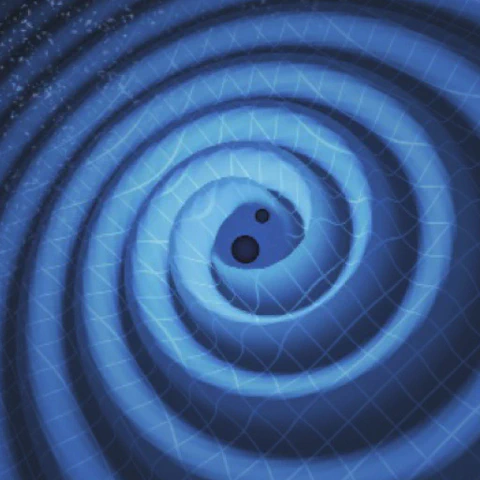
Code for solving the coagulation equation for black hole and neutron star mergers in dense clusters and predicting the observed black hole mass function by gravitational-wave detectors. The main equation that the code solves is the discrete coagulation (Smoluchowski) equation, $$\dot N_i=\frac{1}{2}\sum_{j=1}^{i-1}R_{i-j,j}N_{i-j}N_j-\sum_{j=1}^{\infty}R_{i,j}N_iN_j.$$Here, $N_i$ is the number of black holes of mass $M_i$ while $R_{i,j}N_iN_j$ is the merger rate of black holes of mass $M_i$ and $M_j$. This first term on the RHS thus increases $N_i$ due to mergers of smaller black holes (that result in a remnant mass of $M_i$), while the second term lowers $N_i$ due to mergers between $M_i$ and any other black hole. This equation however needs to be modified in order to simulate a realistic cluster dynamics, since it implictly assumes that all black holes remain in the cluster, that there is no mass loss due to gravitational-wave emission, and that the mergers happen instantaneously once a black hole binary was formed. See more information at arxiv: 2008.10389. Let us assume for example that we have a cluster that initially contains 300 black holes of different masses. The following plots show the total number and total mass of the black holes in the cluster, with different ejection models. In all models, the total number of black holes decreases over time (due to mergers) as well as the total mass (unless there are no ejections). We can also study how different interaction rates affect the final black hole mass function and the probability for intermediate-mass black hole (IMBH) formation, this is a black hole of mass greater than 500 solar masses. In the plots below, the interaction rate is modeled as $R_{i,j}\propto\left(\frac{\min\left(M_i,M_j\right)}{\max\left(M_i,M_j\right)}\right)^\beta\left(M_i+M_j\right)^{\gamma}$, and $\beta$ and $\gamma$ are zero, unless the legend says otherwise. Interestingly, while positive $\gamma$ and negative $\beta$ models allow IMBH fromation, the final black hole mass function looks very different!