SPaRTA

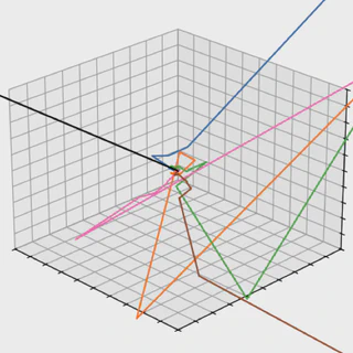
SPaRTA 🛡️ = SPeedy Lyman alpha Ray Tracing Algorithm. The code can be used to perform quickly MC simulations of the trajectories of absorbed Lyman alpha photons in the intergalactic medium (IGM), plotting them, and gather insights on their properties.

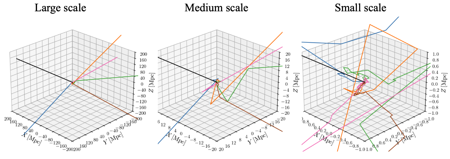
Let us look for example on the trajectories of 6 photons as they travel through the IGM, until they are absorbed at the center at redshift $z_\mathrm{abs}=10$. The black line in all plots corresponds to a photon traveling in a straight-line. On large scales, all photons appear to travel in straight-lines as their aparent frequency is far away from the Lyman alpha line center. On small scales, the photons appear to do a random walk with a step size that decreases as we zoom-in, this happens as on the smallest scales the frequency of the photons is close to Lyman alpha and the cross-section for interacting with the hydrogen atoms in the IGM becomes very large.

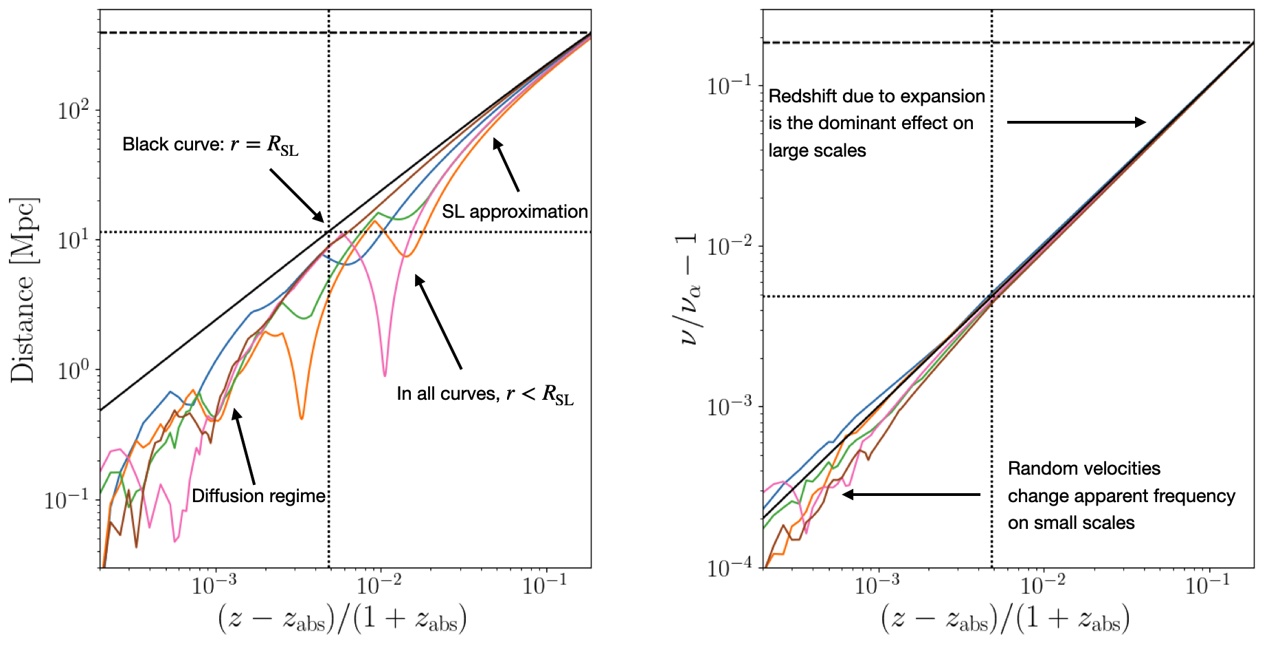
The diffustion scale is the intermediate scale that separates “large” scales and “small” scales. It can be analytically estimated to be

$$r_{*}\left(z_\mathrm{abs}\right)\approx10\,x_{\mathrm{HI}}\left(\frac{\Omega_{b}h^{2}}{0.0223}\right)\left(\frac{\Omega_{m}h^{2}}{0.143}\right)^{-1}\left(\frac{1-Y_{\mathrm{He}}}{0.755}\right)\left(\frac{1+z_{\mathrm{abs}}}{10}\right)\,\mathrm{Mpc}.$$

We can see indeed that the photons change their behavior when we plot their distance and frequency from the origin as a function of time (or redshift). The dotted lines below mark the diffusion scale.

Interstingly, when studying the radial distribution of the photons from the origin, given absorption redshift $z_\mathrm{abs}$ and emission redshift $z_\mathrm{em}$, the distribution depends mainly on $x_\mathrm{em}\equiv R_\mathrm{SL}\left(z_\mathrm{abs},z_\mathrm{em}\right)/r_{*}\left(z_\mathrm{abs}\right)$, where $R_\mathrm{SL}\left(z_\mathrm{abs},z_\mathrm{em}\right)$ is the comoving distance between $z_\mathrm{abs}$ and $z_\mathrm{em}$. This quantity can be thought of as the comoving distance between absorber and emitter, normalized by the diffusion scale. So for $x_\mathrm{em}\gg 1$, the distribution tends towards $\delta\left(r-R_\mathrm{SL}\right)$, reflecting the straight-line limit, while for $x_\mathrm{em}\ll 1$, the distribution shifts more towards smaller distances.

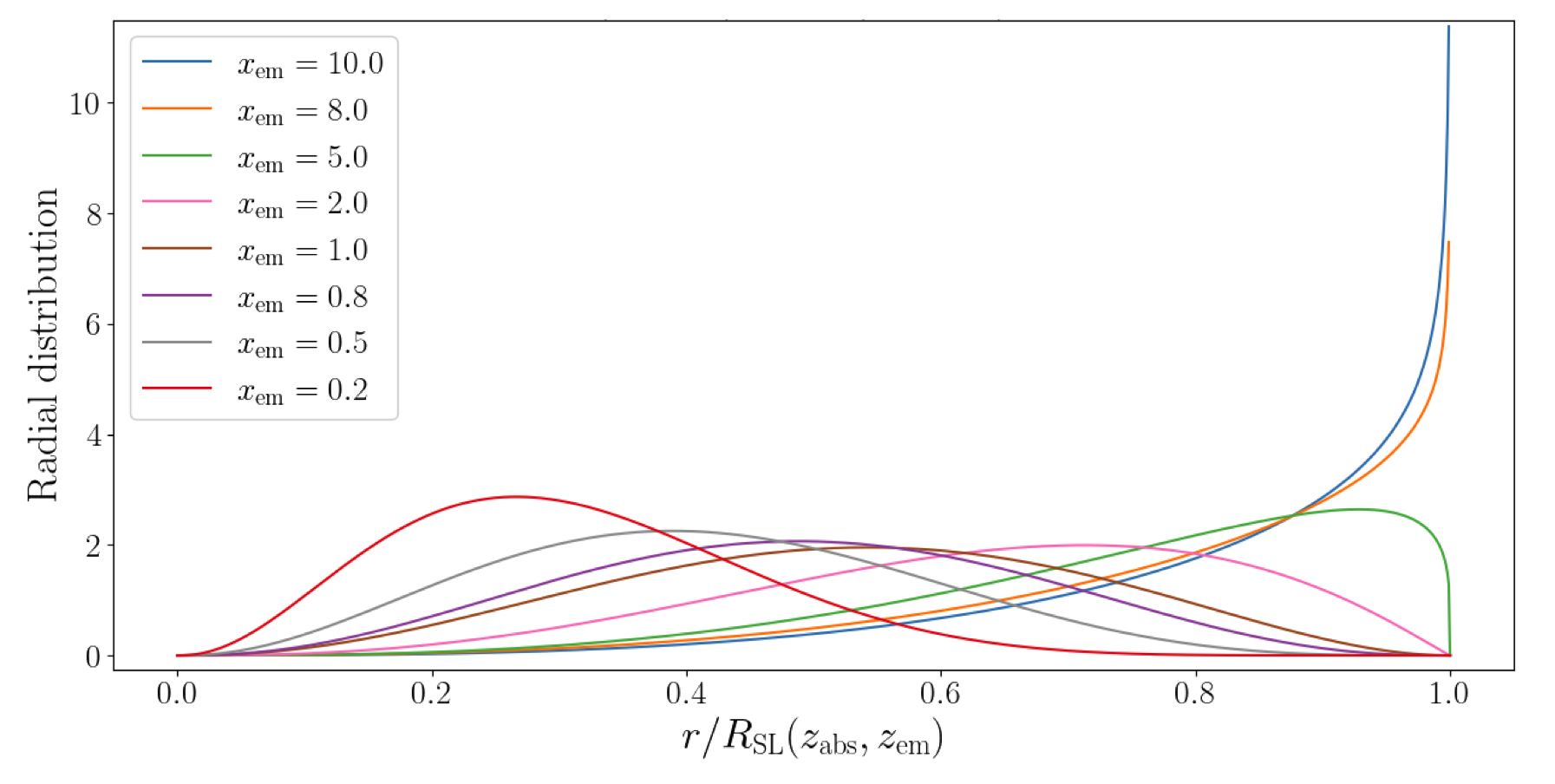
These distributions can be fitted nicely to beta distributions, $f\left(r\right)\propto r^{\alpha-1}\left(R_\mathrm{SL}-r\right)^{\beta-1}$. When $x_\mathrm{em}\gg 1$ we have $\alpha\gg\beta$, while $x_\mathrm{em}\ll 1$ corresponds to $\alpha\ll\beta$.